
2.4: The Real Zeros of a Polynomial Function
Learning Objectives
- Evaluate a polynomial using the Remainder Theorem.
- Find the potential zeros of a polynomial.
- Use the Rational Zero Theorem to find rational zeros.
- Use of synthetic division to divide polynomials.
- Find zeros of a polynomial function.
Evaluate a polynomial using the Remainder Theorem
Polynomials using the Remainder Theorem. If the polynomial is divided by [latex]x–k[/latex], the remainder may be found quickly by evaluating the polynomial function at [latex]k[/latex], that is, [latex]f\left(k\right)[/latex]. Let’s walk through the proof of the theorem.
Recall that the Division Algorithm states that, given a polynomial dividend [latex]f\left(x\right)[/latex] and a non-zero polynomial divisor [latex]d\left(x\right)[/latex], there exist unique polynomials [latex]q\left(x\right)[/latex] and [latex]r\left(x\right)[/latex] such that
[latex]f\left(x\right)=d\left(x\right)q\left(x\right)+r\left(x\right)[/latex]
and either [latex]r\left(x\right)=0[/latex] or the degree of [latex]r\left(x\right)[/latex] is less than the degree of [latex]d\left(x\right)[/latex]. In practice divisors, [latex]d\left(x\right)[/latex] will have degrees less than or equal to the degree of [latex]f\left(x\right)[/latex]. If the divisor, [latex]d\left(x\right)[/latex], is [latex]x−k[/latex], this takes the form
[latex]f\left(x\right)=\left(x-k\right)q\left(x\right)+r[/latex]
Since the divisor [latex]x−k[/latex] is linear, the remainder will be a constant, [latex]r[/latex]. And, if we evaluate this for [latex]x=k[/latex], we have
[latex]f\left(k\right)=\left(k-k\right)q\left(k\right)+r[/latex]
[latex]=0\cdot q\left(k\right)+r[/latex]
[latex]=r[/latex]
In other words, [latex]f\left(k\right)[/latex] is the remainder obtained by dividing [latex]f\left(x\right)[/latex] by [latex]x−k[/latex].
The Remainder Theorem
If a polynomial [latex]f\left(x\right)[/latex] is divided by [latex]x−k[/latex], then the remainder is the value [latex]f\left(k\right)[/latex].
How To
Given a polynomial function [latex]f[/latex], evaluate [latex]f\left(x\right)[/latex] at [latex]x=k[/latex] using the Remainder Theorem.
- Use synthetic division to divide the polynomial by [latex]x−k[/latex].
- The remainder is the value [latex]f\left(k\right)[/latex].
Example 2.4-1-1: Using the Remainder Theorem to Evaluate a Polynomial
Use the Remainder Theorem to evaluate [latex]f\left(x\right)=6x^4-x^3-15x^2+2x-7[/latex] at [latex]x=2[/latex].
 Key
Key
Example 2.4-1-1: Using the Remainder Theorem to Evaluate a Polynomial
Use the Remainder Theorem to evaluate [latex]f\left(x\right)=6x^4-x^3-15x^2+2x-7[/latex] at [latex]x=2[/latex].
We can check our answer by evaluating [latex]f\left(2\right)[/latex].
[latex]f\left(x\right)=6x^4-x^3-15x^2+2x-7[/latex]
[latex]f\left(2\right)=6\left(2\right)^4-\left(2\right)^3-15\left(2\right)^2+2\left(2\right)-7[/latex]
[latex]=25[/latex]
Your Turn
Practice 2.4-1-1
Find the potential zeros of a polynomial
The Rational Zero Theorem
The Rational Zero Theorem states that, if the polynomial [latex]f\left(x\right)=a_nx^n+a_{n-1}x^{n-1}+\dots+a_1x+a_0[/latex] has integer coefficients [latex]a_n\neq0[/latex], then every rational zero of [latex]f\left(x\right)[/latex] has the form [latex]\frac pq[/latex] where [latex]p[/latex] is a factor of the constant term [latex]a_0[/latex] and [latex]q[/latex] is a factor of the leading coefficient [latex]a_n[/latex].
When the leading coefficient is [latex]1[/latex], the possible rational zeros are the factors of the constant term.
How To
Given a polynomial function [latex]f\left(x\right)[/latex], use the Rational Zero Theorem to find rational zeros.
- Determine all factors of the constant term and all factors of the leading coefficient.
- Determine all possible values of [latex]\frac pq[/latex], where [latex]p[/latex] is a factor of the constant term and [latex]q[/latex] is a factor of the leading coefficient. Be sure to include both positive and negative candidates.
- Determine which possible zeros are actual zeros by evaluating each case of [latex]f\left(\frac pq\right)[/latex]
Example 2.4-2-1: Listing All Possible Rational Zeros
List all possible rational zeros of [latex]f\left(x\right)=2x^4-5x^3+x^2-4[/latex].
Key
Example 2.4-2-1: Listing All Possible Rational Zeros
List all possible rational zeros of [latex]f\left(x\right)=2x^4-5x^3+x^2-4[/latex].
The only possible rational zeros of [latex]f\left(x\right)[/latex] are the quotients of the factors of the last term, [latex]–4[/latex], and the factors of the leading coefficient, [latex]2[/latex].
The constant term is [latex]–4[/latex]; the factors of [latex]–4[/latex] are [latex]p=\pm1,\;\pm2,\;\pm4[/latex].
The leading coefficient is [latex]2[/latex]; the factors of [latex]2[/latex] are [latex]q=\pm1,\;\pm2[/latex].
If any of the four real zeros are rational zeros, then they will be of one of the following factors of [latex]–4[/latex] divided by one of the factors of [latex]2[/latex].
|
[latex]\frac pq=\pm\frac11,\;\pm\frac12[/latex] |
[latex]\frac pq=\pm\frac21,\;\pm\frac22[/latex] |
[latex]\frac pq=\pm\frac41,\;\pm\frac42[/latex] |
Note that [latex]\frac22=1[/latex] and [latex]\frac42=2[/latex], which have already been listed. So we can shorten our list.
[latex]\frac pq=\frac{Factors\;of\;the\;last}{Factors\;of\;the\;first}=\pm1,\;\pm2,\;\pm4,\;\pm\frac12[/latex]
 Your Turn
Practice 2.4-2-1
Use the Rational Zero Theorem to find rational zero
To find rational zeros of a polynomial
- First, list all possible (potential) rational zeros.
- Then, use the Remainder Theorem to test them.
If substituting a value for [latex]x[/latex] results in a remainder of [latex]0[/latex], that value is a real zero of the polynomial.
Example 2.4-3-1: Using the rational zero theorem to final rational zeros.
[latex]f\left(x\right)=2x^4-5x^3+x^2-4[/latex]
Key
Example 2.4-3-1: Using the rational zero theorem to final rational zeros.
[latex]f\left(x\right)=2x^4-5x^3+x^2-4[/latex]
Step 1: Find all potential zeros.
From Example 2.4-2-1 we have found the potential zeros
[latex]\frac pq=\pm1,\;\pm2,\;\pm4,\;\pm\frac12[/latex]
Step 2: use the Remainder Theorem to test them.
[latex]f\left(1\right)=2\left(1\right)^4-5\left(1\right)^3+\left(1\right)^2-4=-6[/latex]
[latex]f\left(-1\right)=2\left(-1\right)^4-5\left(-1\right)^3+\left(-1\right)^2-4=4[/latex]
[latex]f\left(-2\right)=2\left(-2\right)^4-5\left(-2\right)^3+\left(-2\right)^2-4=72[/latex]
[latex]f\left(2\right)=2\left(2\right)^4-5\left(2\right)^3+\left(2\right)^2-4=-8[/latex]
[latex]f\left(-4\right)=2\left(-4\right)^4-5\left(-4\right)^3+\left(-4\right)^2-4=844[/latex]
[latex]f\left(4\right)=2\left(4\right)^4-5\left(4\right)^3+\left(4\right)^2-4=204[/latex]
[latex]f\left(\frac12\right)=2\left(\frac12\right)^4-5\left(\frac12\right)^3+\left(\frac12\right)^2-4=-\frac{17}4[/latex]
[latex]f\left(-\frac12\right)=2\left(-\frac12\right)^4-5\left(-\frac12\right)^3+\left(-\frac12\right)^2-4=-3[/latex]
None of the rational candidates work. That means this polynomial has no rational real zeros.
Your Turn
Practice 2.4-3-1
Use of synthetic division to divide polynomials
As we’ve seen, long division of polynomials can involve many steps and be quite cumbersome. Synthetic division is a shorthand method of dividing polynomials for the special case of dividing by a linear factor whose leading coefficient is [latex]1[/latex].
To illustrate the process, recall the example at the beginning of the section.
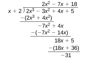
Divide [latex]2x^3-3x^2+4x+5[/latex] by [latex]x+2[/latex] using the long division algorithm.
The final form of the process looked like this:
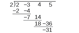
There is a lot of repetition in the table. If we don’t write the variables but, instead, line up their coefficients in columns under the division sign and also eliminate the partial products, we already have a simpler version of the entire problem.
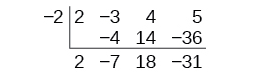
Synthetic division carries this simplification even a few more steps. Collapse the table by moving each of the rows up to fill any vacant spots. Also, instead of dividing by [latex]2[/latex], as we would in division of whole numbers, then multiplying and subtracting the middle product, we change the sign of the “divisor” to [latex]–2[/latex], multiply and add. The process starts by bringing down the leading coefficient.
Synthetic Division
Synthetic division is a shortcut that can be used when the divisor is a binomial in the form [latex]x−k[/latex] where [latex]k[/latex] is a real number. In synthetic division, only the coefficients are used in the division process.
How To
Given two polynomials, use synthetic division to divide.
- Write [latex]k[/latex] for the divisor.
- Write the coefficients of the dividend.
- Bring the lead coefficient down.
- Multiply the lead coefficient by [latex]k[/latex]. Write the product in the next column.
- Add the terms of the second column.
- Multiply the result by [latex]k[/latex]. Write the product in the next column.
- Repeat steps 5 and 6 for the remaining columns.
- Use the bottom numbers to write the quotient. The number in the last column is the remainder. The next number from the right has degree [latex]0[/latex], the next number has degree [latex]1[/latex], and so on.
Example 2.4-4-1: Using Synthetic Division to Divide a Second-Degree Polynomial
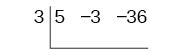
Use synthetic division to divide [latex]5x^2-3x-36[/latex] by [latex]x-3[/latex].
Key
Example 2.4-4-1: Using Synthetic Division to Divide a Second-Degree Polynomial
Use synthetic division to divide [latex]5x^2-3x-36[/latex] by [latex]x-3[/latex].
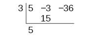
Begin by setting up the synthetic division. Write [latex]k[/latex] and the coefficients.
Bring down the lead coefficient. Multiply the lead coefficient by [latex]k[/latex].
Continue by adding the numbers in the second column. Multiply the resulting number by [latex]k[/latex]. Write the result in the next column. Then add the numbers in the third column.
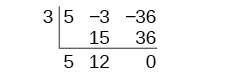
The result is [latex]5x+12[/latex]. The remainder is [latex]0[/latex]. So [latex]x−3[/latex] is a factor of the original polynomial.
Just as with long division, we can check our work by multiplying the quotient by the divisor and adding the remainder.
[latex]\left(x-3\right)\left(5x+12\right)+0=5x^2-3x-36[/latex]
Find zeros of a polynomial function
Steps to Find Real Zeros of a Polynomial
- List possible rational zeros
[latex]\frac pq=\pm\frac{factors\;of\;cons\tan t}{factors\;of\;leading\;coefficient}[/latex]
- Test values using Remainder Theorem
Plug into the polynomial.
If [latex]f\left(x\right)=0[/latex], then x is a real zero. - Use Synthetic Division
Divide the polynomial by opposite value of x (real zero).
This gives a simpler polynomial. Repeat the process. - Solve the remaining polynomial
Factor or use the quadratic formula to find more zeros.
Example 2.4-5-1: Find zeros of a polynomial function
[latex]f\left(x\right)=x^3-6x^2+11x-6[/latex]
Key
Example 2.4-4-1: Find zeros of a polynomial function
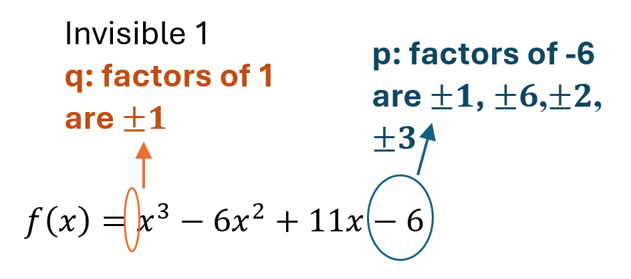
- List possible rational zeros
[latex]\frac pq=\pm\frac{factors\;of\;cons\tan t}{factors\;of\;leading\;coefficient}[/latex]
[latex]\frac pq=\pm\frac11,\;\pm\frac61,\;\pm\frac21,\;\pm\frac31[/latex]
[latex]\frac pq=\pm1,\;\pm6,\;\pm2,\;\pm3[/latex]
- Test values using Remainder Theorem
Plug into the polynomial.
If [latex]f\left(x\right)=0[/latex], then [latex]x[/latex] is a real zero.
Test values if [latex]x=1[/latex]
[latex]f\left(1\right)=\left(1\right)^3-6\left(1\right)^2+11\left(1\right)-6=0[/latex]
Once we find one real zero, we can stop at this step and start the next step.
[latex]x=1[/latex]
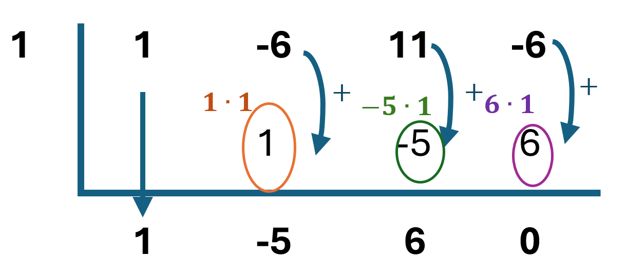
- Use Synthetic Division
Divide the polynomial by the value of [latex]x[/latex] we found in step 2 (real zero).
This gives a simpler polynomial. Repeat the process.
- Solve the remaining polynomial
Factor or use the quadratic formula to find more zeros.
[latex]x^2-5x+6=0[/latex]
[latex]\left(x-2\right)\left(x-3\right)=0[/latex]
[latex]x=2,\;x=3[/latex]
Overall real zeros are: [latex]x=1,\;x=2,\;x=3[/latex]
Your Turn
Practice 2.4-5-1
Licenses and Attribution
CC Licensed Content
- College-algebra-2e by Jay Abramson is licensed CC BY. Access for free.
