
1.5: Graphing techniques: transformations; solving radical equations
Learning Objectives
- Graph functions using vertical and horizontal shifts.
- Graph functions using compressions and stretches.
- Graph functions using reflections about the axes.
- Find the equation of function from the transformations.
Graphing Functions Using Vertical And Horizontal Shifts
Vertical Shift
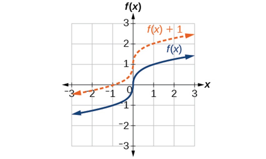
Given a function [latex]f\left(x\right)[/latex], a new function [latex]g\left(x\right)=f\left(x\right)+k[/latex], where [latex]k[/latex] is a constant, is a vertical shift of the function [latex]f\left(x\right)[/latex]. All the output values change by [latex]k[/latex] units. If [latex]k[/latex] is positive, the graph will shift up. If [latex]k[/latex] is negative, the graph will shift down.
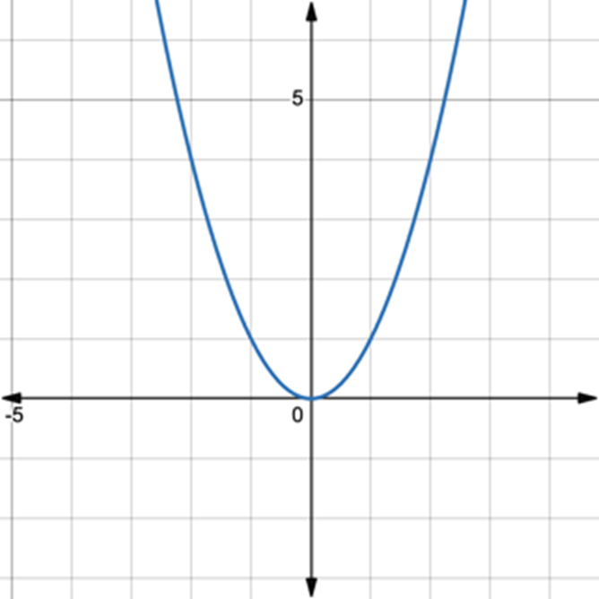
Example 1.5-1-1: Given the graph [latex]f\left(x\right)=x^2[/latex], graph the transformed function: [latex]f\left(x\right)=x^2+2[/latex].
[latex]f\left(x\right)=x^2[/latex]
 Key
Key
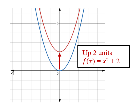
Example 1.5-1-1: Given the graph [latex]f\left(x\right)=x^2[/latex], graph the transformed function: [latex]f\left(x\right)=x^2+2[/latex]
[latex]f\left(x\right)=x^2[/latex]
If the whole function [latex]f\left(x\right)[/latex] changes, then up or down. [latex]k[/latex] is 2 which is positive, the graph will shift up 2 units.
Horizontal Shift
Given a function [latex]f[/latex],a new function [latex]g\left(x\right)=f\left(x-h\right)[/latex], where [latex]h[/latex] is a constant, is a horizontal shift of the function [latex]f[/latex]. If [latex]h[/latex] is positive, the graph will shift right. If [latex]h[/latex] is negative, the graph will shift left.
Example 1.5-1-2: Given the graph [latex]f\left(x\right)=x^2[/latex], graph the transformed function: [latex]f\left(x\right)=\left(x+2\right)^2[/latex].
Key
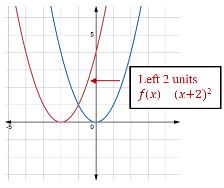
Example 1.5-1-2: Given the graph [latex]f\left(x\right)=x^2[/latex], graph the transformed function: [latex]f\left(x\right)=\left(x+2\right)^2[/latex]
[latex]f\left(x\right)=x^2[/latex]
[latex]f\left(x\right)=\left(x+2\right)^2[/latex]
The change relates to x, and since function f\left(x\right)=\left(x-\left(-2\right)\right)^2 where [latex]h[/latex] is -2, [latex]h[/latex] is negative, the graph will shift left 2 units.
Graphing Functions Using Compressions And Stretches
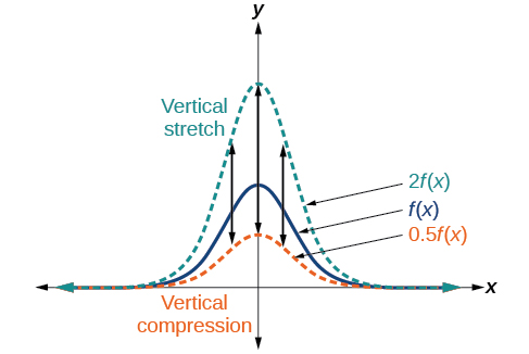
Vertical Stretches and Compressions
Given a function [latex]f\left(x\right)[/latex], a new function [latex]g\left(x\right)=af\left(x\right)[/latex], where a is a constant, is a vertical stretch or vertical compression of the function [latex]f\left(x\right)[/latex].
- If [latex]a>1[/latex], then the graph will be stretched.
- If 0 < a < 1, then the graph will be compressed.
- If [latex]a<0[/latex], then there will be combination of a vertical stretch or compression with a vertical reflection.
Steps:
Given a function, graph its vertical stretch.
- Identify the value of [latex]a[/latex].
- Multiply all range values by [latex]a[/latex].
- If [latex]a>1[/latex], the graph is stretched by a factor of a.
If 0 < a < 1, the graph is compressed by a factor of a.
If [latex]a<0[/latex], the graph is either stretched or compressed and also reflected about the x-axis.
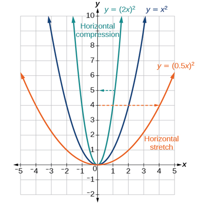
Horizontal Stretches and Compressions
Given a function [latex]f\left(x\right)[/latex], a new function [latex]g\left(x\right)=f\left(bx\right)[/latex], where [latex]b[/latex] is a constant, is a horizontal stretch or horizontal compression of the function [latex]f\left(x\right)[/latex].
- If [latex]b>1[/latex], then the graph will be compressed by [latex]b[/latex].
- If 0 < b < 1, then the graph will be stretched by [latex]\frac1b[/latex].
- If [latex]b<0[/latex], then there will be combination of a horizontal stretch or compression with a horizontal reflection.
Steps:
Given a description of a function, sketch a horizontal compression or stretch.
- Write a formula to represent the function.
- Set [latex]g\left(x\right)=f\left(bx\right)[/latex] where [latex]b >1[/latex] for a compression or 0 < b < 1 for a stretch.
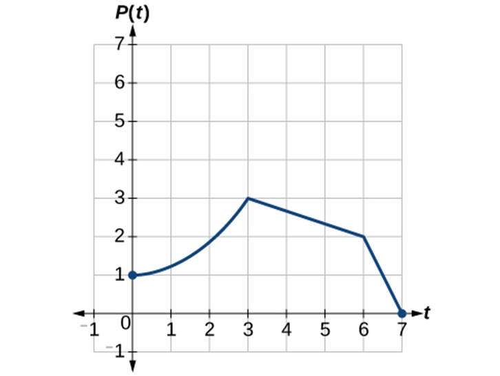
Example 1.5-2-1: Given the graph, graph the transformed function
Key
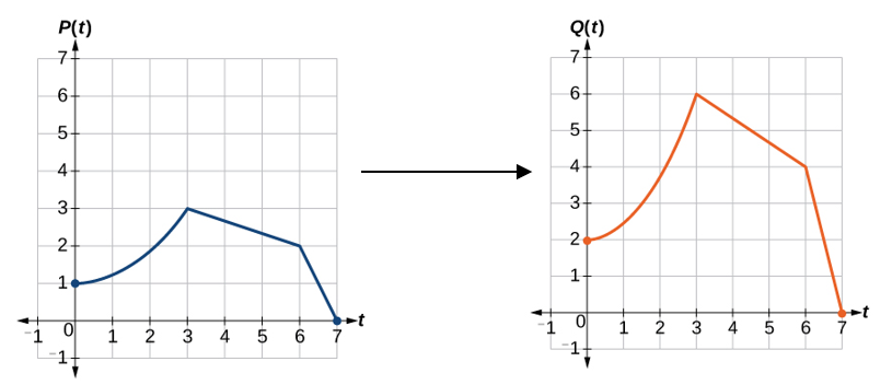
Example 1.5-2-1: Given the graph, graph the transformed function
If we choose four reference points, (0, 1), (3, 3), (6, 2) and (7, 0) … …
[latex]\left(7,\;0\right)\rightarrow\left(7,\;0\right)[/latex]
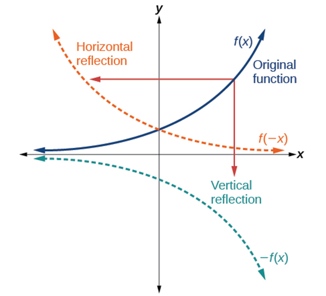
Graphing Functions Using Reflections About the Axes
Reflections
Given a function [latex]f\left(x\right)[/latex], a new function [latex]g\left(x\right)=-f\left(x\right)[/latex] is a vertical reflection of the function [latex]f\left(x\right)[/latex], sometimes called a reflection about (or over, or through) the x-axis.
Given a function [latex]f\left(x\right)[/latex], a new function [latex]g\left(x\right)=f\left(-x\right)[/latex] is a horizontal reflection of the function [latex]f\left(x\right)[/latex], sometimes called a reflection about the y-axis.
Steps:
Given a function, reflect the graph both vertically and horizontally.
- Multiply all outputs by –1 for a vertical reflection. The new graph is a reflection of the original graph about the x-axis.
- Multiply all inputs by –1 for a horizontal reflection. The new graph is a reflection of the original graph about the y-axis.
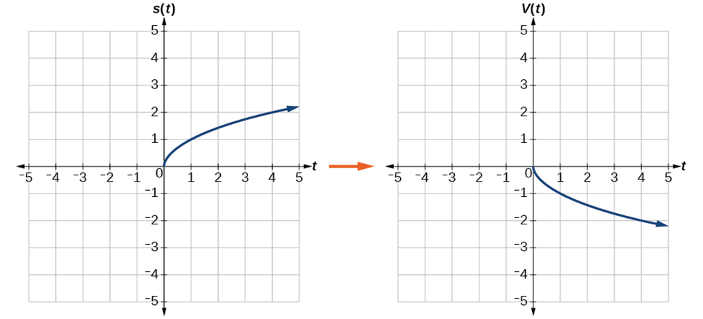
Example 1.5-3-1: Given the graph [latex]s\left(t\right)=\sqrt t[/latex], graph the transformed function [latex]v\left(t\right)=-\sqrt t[/latex]
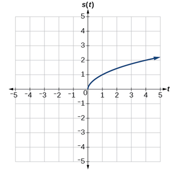
Key
Example 1.5-3-1: Given the graph [latex]s\left(t\right)=\sqrt t[/latex], graph the transformed function [latex]v\left(t\right)=-\sqrt t[/latex]
Because each output value is the opposite of the original output value, we can write
[latex]V\left(t\right)=-s\left(t\right)\;or\;V\left(t\right)=-\sqrt t[/latex]
 Your Turn
Practice 1.5-3-1
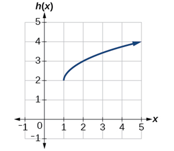
Example 1.5-4-1: Identify combined vertical and horizontal shift and write the transformed function.
Key
Example 1.5-4-1: Identify combined vertical and horizontal shift and write the transformed function.
Based on the given graph, we can tell that it represents a square root function. First, we need to identify the parent graph—the original graph. Then, by comparing it with the transformed graph, we can determine the movement.
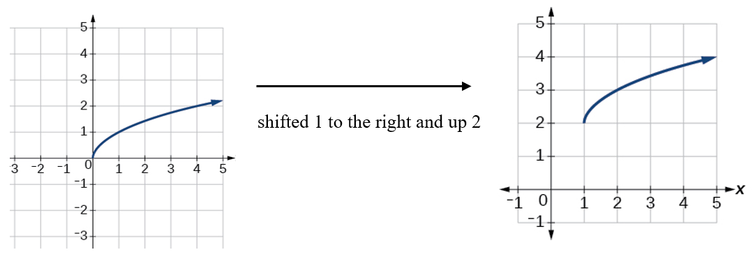
Using the formula for the square root function, we can write
[latex]h\left(x\right)=\sqrt x\xrightarrow[{shifted\;1\;unit\;to\;the\;right\;}]{}\sqrt{x-1}\xrightarrow[{up\;2\;units\;}]{}\sqrt{x-1}+2[/latex]
Answer: [latex]h\left(x\right)=\sqrt{x-1}+2[/latex]
Licenses and Attribution
CC Licensed Content
- Precalculus-2e by Jay Abramson is licensed CC BY. Access for free.
