2.3: Polynomial Functions and Models
Learning Objectives
- Identify Polynomial Functions and Their Degree
- Identify the Real Zeros of a Polynomial Function and Their Multiplicity
- Analyze the Graph of a Polynomial Function
Identify Polynomial Functions and Their Degree
Polynomials
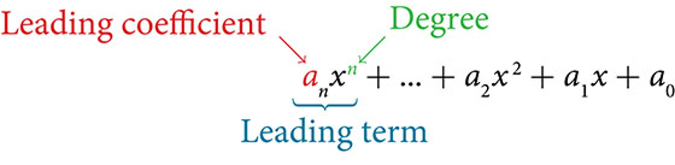
A polynomial is an expression that can be written in the form
[latex]a_nx^n+\dots a_2x^2+a_1x+a_0[/latex]
Each real number ai is called a coefficient. The number [latex]a_0[/latex] that is not multiplied by a variable is called a constant. Each product [latex]a_ix^i[/latex] is a term of a polynomial. The highest power of the variable that occurs in the polynomial is called the degree of a polynomial. The leading term is the term with the highest power, and its coefficient is called the leading coefficient.
Steps
Given a polynomial expression, identify the degree and leading coefficient.
- Find the highest power of [latex]x[/latex] to determine the degree.
- Identify the term containing the highest power of [latex]x[/latex] to find the leading term.
- Identify the coefficient of the leading term.
Example 2.3-1-1: Identifying the Degree and Leading Coefficient of a Polynomial
For the following polynomials, identify the degree, the leading term, and the leading coefficient.
- [latex]3+2x^2-4x^3[/latex]
- [latex]5t^5-2t^3+7t[/latex]
- [latex]6p-p^3-2[/latex]
 Key
Key
Example 2.3-1-1: Identifying the Degree and Leading Coefficient of a Polynomial
For the following polynomials, identify the degree, the leading term, and the leading coefficient.
- [latex]3+2x^2-4x^3[/latex]
- [latex]5t^5-2t^3+7t[/latex]
- [latex]6p-p^3-2[/latex]
Solution
- The highest power of [latex]x[/latex] is [latex]3[/latex], so the degree is [latex]3[/latex]. The leading term is the term containing that degree, [latex]-4x^3[/latex]. The leading coefficient is the coefficient of that term, [latex]−4[/latex].
- The highest power of [latex]t[/latex] is [latex]5[/latex], so the degree is [latex]5[/latex]. The leading term is the term containing that degree, [latex]5t^5[/latex]. The leading coefficient is the coefficient of that term, [latex]5[/latex].
- The highest power of [latex]p[/latex] is [latex]3[/latex], so the degree is [latex]3[/latex]. The leading term is the term containing that degree, [latex]-p^3[/latex], The leading coefficient is the coefficient of that term, [latex]−1[/latex].
 Your Turn
Practice 2.3-1-1
Identify the Real Zeros of a Polynomial Function and Their Multiplicity
Multiplicity:
If [latex]\left(x-r\right)^m[/latex] is a factor of a polynomial [latex]f[/latex] and [latex]\left(x-r\right)^{m+1}[/latex] is not a factor of [latex]f[/latex], then [latex]r[/latex] is called a real zero of multiplicity [latex]m[/latex] of [latex]f[/latex].
Format:
[latex]f\left(x\right)=\left(x-r_1\right)^{m_1}\left(x-r_2\right)^{m_2}\left(x-r_3\right)^{m_3}\cdots\;\cdots\left(x-r_{n-1}\right)^{m_{n-1}}\left(x-r_n\right)^{m_n}[/latex]
If [latex]r_1\neq r_2\neq r_3\neq\cdots r_{n-1}\neq r_n[/latex]
In this format,
[latex]m_1,\;m_2,\;m_3\;\dots\;\dots\;m_{n-1},\;m_n[/latex] are the multiplicities.
Turning Points:
The most turning points = The highest degree of the polynomial-1
Real Zeros:
If [latex]f[/latex] is a function and [latex]r[/latex] is a real number for which [latex]f\left(r\right)=0[/latex], then [latex]r[/latex] is called a real zero of [latex]f[/latex].
Thus: [latex]r[/latex] is a real zero of a polynomial function [latex]f = r[/latex] is an x-intercept of the graph of [latex]f = r[/latex] is a real solution to the equation [latex]f\left(x\right)=0[/latex]
Format:
[latex]f\left(x\right)=\left(x-r_1\right)^{m_1}\left(x-r_2\right)^{m_2}\left(x-r_3\right)^{m_3}\cdots\;\cdots\left(x-r_{n-1}\right)^{m_{n-1}}\left(x-r_n\right)^{m_n}[/latex]
If [latex]r_1\neq r_2\neq r_3\neq\cdots r_{n-1}\neq r_n[/latex]
In this format,
[latex]r_1,\;r_2,\;r_3\;\dots\;\dots\;r_{n-1},\;r_n[/latex] are real zeros of the polynomials.
Example 2.3-2-1: Using the given polynomial, find the degree, leading term, leading coefficient, multiplicity, maximum number of turning points, and real zeros.
[latex]f\left(x\right)=3\left(x-4\right)\left(x-1\right)^2[/latex]
Key
Example 2.3-2-1: Using the given polynomial, find the degree, leading term, leading coefficient, multiplicity, maximum number of turning points, and real zeros.
[latex]f\left(x\right)=3\left(x-4\right)\left(x-1\right)^2[/latex]
Degree:
To find degree, we just need to find the highest power of the x in the expanded form. We have
[latex]f\left(x\right)=3\left(x-4\right)\left(x-1\right)^2[/latex]
[latex]f\left(x\right)=3\left(x-4\right)\left(x^2-2x+1\right)[/latex]
[latex]f\left(x\right)=\left(3x-12\right)\left(x^2-2x+1\right)[/latex]
[latex]f\left(x\right)=3x^3-6x^2-3x-12x^2+24x-12[/latex]
[latex]\begin{array}{c}f\left(x\right)=\boxed{3x^{\color[rgb]{0.5, 0.0, 0.5}\mathbf3}}-18x^2+21x-12\\\!\\\color[rgb]{0.5, 0.0, 0.5}\boxed{\mathbf T\mathbf h\mathbf e\boldsymbol\;\mathbf h\mathbf i\mathbf g\mathbf h\mathbf e\mathbf s\mathbf t\boldsymbol\;\mathbf d\mathbf e\mathbf g\mathbf r\mathbf e\mathbf e\boldsymbol\;\mathbf o\mathbf f\boldsymbol\;\mathbf t\mathbf h\mathbf e\boldsymbol\;\mathbf p\mathbf o\mathbf l\mathbf y\mathbf n\mathbf o\mathbf m\mathbf i\mathbf a\mathbf l}\end{array}[/latex]
Degree is [latex]3[/latex].
Leading Term:
Since the highest degree of [latex]x[/latex] is [latex]3[/latex], the term that contains [latex]x^3[/latex] is the leading term.
Leading term: [latex]3x^3[/latex].
Leading Coefficient:
Since the leading term is [latex]3x^3[/latex], the coefficient of the leading term is the leading coefficient.
Leading coefficient: [latex]3[/latex].
Multiplicity:
If [latex]\left(x-r\right)^m[/latex] is a factor of a polynomial [latex]f[/latex] and [latex]\left(x-r\right)^{m+1}[/latex] is not a factor of [latex]f[/latex], then [latex]r[/latex] is called a real zero of multiplicity [latex]m[/latex] of [latex]f[/latex].
Format:
[latex]f\left(x\right)=\left(x-r_1\right)^{m_1}\left(x-r_2\right)^{m_2}\left(x-r_3\right)^{m_3}\cdots\;\cdots\left(x-r_{n-1}\right)^{m_{n-1}}\left(x-r_n\right)^{m_n}[/latex]
[latex]m_1,\;m_2,\;m_3\;\dots\;\dots\;m_{n-1},\;m_n[/latex] are the multiplicities.
In this question we have
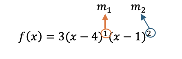
Thus [latex]m_1=1,\;m_2=2[/latex]
Turning Points:
The most turning points = The highest degree of the polynomial-1
The most turning points = [latex]3 – 1 = 2[/latex]
Real Zeros:
If [latex]f[/latex] is a function and [latex]r[/latex] is a real number for which [latex]f\left(r\right)=0[/latex], then [latex]r[/latex] is called a real zero of [latex]f[/latex].
Thus: [latex]r[/latex] is a real zero of a polynomial function [latex]f = r[/latex] is an x-intercept of the graph of [latex]f = r[/latex] is a real solution to the equation [latex]f\left(x\right)=0[/latex]
Format:
[latex]f\left(x\right)=\left(x-r_1\right)^{m_1}\left(x-r_2\right)^{m_2}\left(x-r_3\right)^{m_3}\cdots\;\cdots\left(x-r_{n-1}\right)^{m_{n-1}}\left(x-r_n\right)^{m_n}[/latex]
[latex]r_1,\;r_2,\;r_3\;\dots\;\dots\;r_{n-1},\;r_n[/latex] are real zeros of the polynomials.
In this question we have
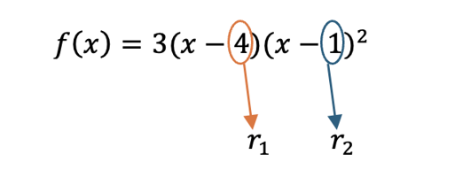
Real zeros are [latex]4[/latex], and [latex]1[/latex].
Your Turn
Practice 2.3-2-1
Analyze the Graph of a Polynomial Function
Graphs of polynomial functions with multiplicity 1, 2, and 3.
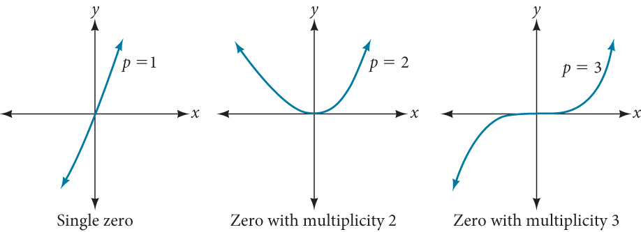
For higher even powers, such as 4, 6, and 8, the graph will still touch and bounce off of the horizontal axis but, for each increasing even power, the graph will appear flatter as it approaches and leaves the x-axis.
For higher odd powers, such as 5, 7, and 9, the graph will still cross through the horizontal axis, but for each increasing odd power, the graph will appear flatter as it approaches and leaves the x-axis.
If a polynomial contains a factor of the form [latex]\left(x-h\right)^p[/latex], the behavior near the x- intercept [latex]h[/latex] is determined by the power p. We say that [latex]x=h[/latex] is a zero of multiplicity [latex]p[/latex].
The graph of a polynomial function will touch the x-axis at zeros with even multiplicities. The graph will cross the x-axis at zeros with odd multiplicities.
The sum of the multiplicities is the degree of the polynomial function.
Given a graph of a polynomial function of degree [latex]n[/latex], identify the zeros and their multiplicities.
- If the graph crosses the x-axis and appears almost linear at the intercept, it is a single zero.
- If the graph touches the x-axis and bounces off of the axis, it is a zero with even multiplicity.
- If the graph crosses the x-axis at a zero, it is a zero with odd multiplicity.
- The sum of the multiplicities is [latex]\leq n[/latex].
Example 2.3-3-1: Identifying Zeros and Their Multiplicities
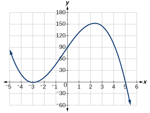
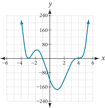
Use the graph of the function of degree 6 in Figure 9 to identify the zeros of the function and their possible multiplicities.
Key
Example 2.3-3-1: Identifying Zeros and Their Multiplicities
Use the graph of the function of degree 6 in Figure 9 to identify the zeros of the function and their possible multiplicities.
The polynomial function is of degree [latex]6[/latex]. The sum of the multiplicities must be [latex]6[/latex].
Starting from the left, the first zero occurs at [latex]x=−3[/latex]. The graph touches the x-axis, so the multiplicity of the zero must be even. The zero of [latex]−3[/latex]
most likely has multiplicity 2.
The next zero occurs at [latex]x=−1[/latex]. The graph looks almost linear at this point. This is a single zero of multiplicity 1.
The last zero occurs at [latex]x=4[/latex]. The graph crosses the x-axis, so the multiplicity of the zero must be odd. We know that the multiplicity is likely [latex]3[/latex] and that the sum of the multiplicities is [latex]6[/latex].
Deterring Ending Behavior
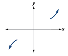
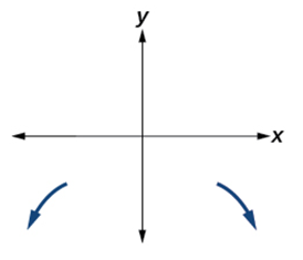
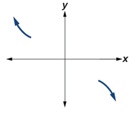
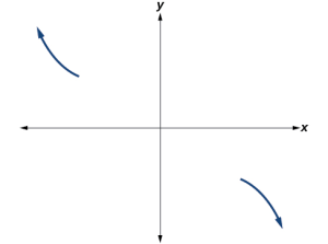
Recall that we call this behavior the end behavior of a function. As we pointed out when discussing quadratic equations, when the leading term of a polynomial function, [latex]a_nx^n[/latex], is an even power function, as [latex]x[/latex] increases or decreases without bound, [latex]f\left(x\right)[/latex] increases without bound. When the leading term is an odd power function, as [latex]x[/latex] decreases without bound, [latex]f\left(x\right)[/latex] also decreases without bound; as [latex]x[/latex] increases without bound, [latex]f\left(x\right)[/latex] also increases without bound. If the leading term is negative, it will change the direction of the end behavior. Figure 11 summarizes all four cases.
| Even Degree | Odd Degree |
|---|---|
| Positive Leading Coefficient, [latex]a_n>0[/latex] | Positive Leading Coefficient, [latex]a_n>0[/latex] |
 |
|
| End Behavior:
[latex]x\rightarrow\infty,\;f\left(x\right)\rightarrow\infty[/latex] [latex]x\rightarrow-\infty,\;f\left(x\right)\rightarrow\infty[/latex] |
End Behavior:
[latex]x\rightarrow\infty,\;f\left(x\right)\rightarrow\infty[/latex] [latex]x\rightarrow-\infty,\;f\left(x\right)\rightarrow-\infty[/latex] |
|
Negative Leading Coefficient, [latex]a_n<0[/latex] |
Negative Leading Coefficient, [latex]a_n<0[/latex] |
 |
 |
| End Behavior:
[latex]x\rightarrow\infty,\;f\left(x\right)\rightarrow-\infty[/latex] [latex]x\rightarrow-\infty,\;f\left(x\right)\rightarrow-\infty[/latex] |
End Behavior:
[latex]x\rightarrow\infty,\;f\left(x\right)\rightarrow-\infty[/latex] [latex]x\rightarrow-\infty,\;f\left(x\right)\rightarrow\infty[/latex] |
Understanding the Relationship between the Turning Points
In addition to the end behavior, recall that we can analyze a polynomial function’s local behavior. It may have a turning point where the graph changes from increasing to decreasing (rising to falling) or decreasing to increasing (falling to rising). Look at the graph of the polynomial function [latex]f\left(x\right)=x^4-x^3-4x^2+4x[/latex] in Figure 12. The graph has three turning points.
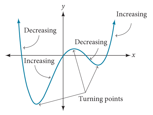
This function [latex]f[/latex] is a 4th degree polynomial function and has 3 turning points. The maximum number of turning points of a polynomial function is always one less than the degree of the function.
Graphing Polynomial Functions
Given a polynomial function, sketch the graph.
- Find the intercepts.
- Check for symmetry. If the function is an even function, its graph is symmetrical about the y-axis, that is, [latex]f\left(-x\right)=f\left(x\right)[/latex]. If a function is an odd function, its graph is symmetrical about the origin, that is, [latex]f\left(-x\right)=f\left(x\right)[/latex].
- Use the multiplicities of the zeros to determine the behavior of the polynomial at the x-
intercepts. - Determine the end behavior by examining the leading term.
- Use the end behavior and the behavior at the intercepts to sketch a graph.
- Ensure that the number of turning points does not exceed one less than the degree of the polynomial.
- Optionally, use technology to check the graph.
Example 2.3-3-2: Sketching the Graph of a Polynomial Function
Sketch a graph of [latex]f\left(x\right)=-2\left(x+3\right)^2\left(x-5\right)[/latex].
Key
Example 2.3-3-2: Sketching the Graph of a Polynomial Function
Sketch a graph of [latex]f\left(x\right)=-2\left(x+3\right)^2\left(x-5\right)[/latex].
This graph has two x-intercepts. At [latex]x=−3[/latex], the factor is squared, indicating a multiplicity of 2. The graph will bounce at this x-intercept. At [latex]x=5[/latex], the function has a multiplicity of one, indicating the graph will cross through the axis at this intercept.
The y-intercept is found by evaluating [latex]f\left(0\right)[/latex].
f\left(0\right)=-2\left(0+3\right)^2\left(0-5\right)
[latex]=-2\cdot9\cdot\left(-5\right)[/latex]
[latex]=90[/latex]
The y-intercept is [latex]\left(0,\;90\right)[/latex].
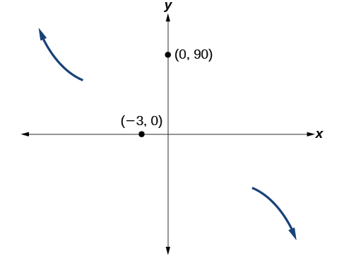
Additionally, we can see the leading term, if this polynomial were multiplied out, would be [latex]-2x^3[/latex], so the end behavior is that of a vertically reflected cubic, with the outputs decreasing as the inputs approach infinity, and the outputs increasing as the inputs approach negative infinity. See Figure 13.
To sketch this, we consider that:
- As [latex]x→−∞[/latex] the function [latex]f\left(x\right)\rightarrow\infty[/latex], so we know the graph starts in the second quadrant and is decreasing toward the x- axis.
- Since [latex]f\left(-x\right)=-2\left(-x+3\right)^2\left(-x-5\right)[/latex] is not equal to [latex]f\left(x\right)[/latex], the graph does not display symmetry.
- At [latex]\left(-3,\;0\right)[/latex], the graph bounces off of the x-axis, so the function must start increasing.
- At [latex]\left(0,\;90\right)[/latex], the graph crosses the y-axis at the y-intercept. See Figure 14.
Somewhere after this point, the graph must turn back down or start decreasing toward the horizontal axis because the graph passes through the next intercept at [latex]\left(5,\;0\right)[/latex]. See Figure 15.
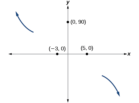
As [latex]x\rightarrow\infty[/latex] the function [latex]f\left(x\right)\rightarrow-\infty[/latex], so we know the graph continues to decrease, and we can stop drawing the graph in the fourth quadrant.
Using technology, we can create the graph for the polynomial function, shown in Figure 16, and verify that the resulting graph looks like our sketch in Figure 15.